Usage¶

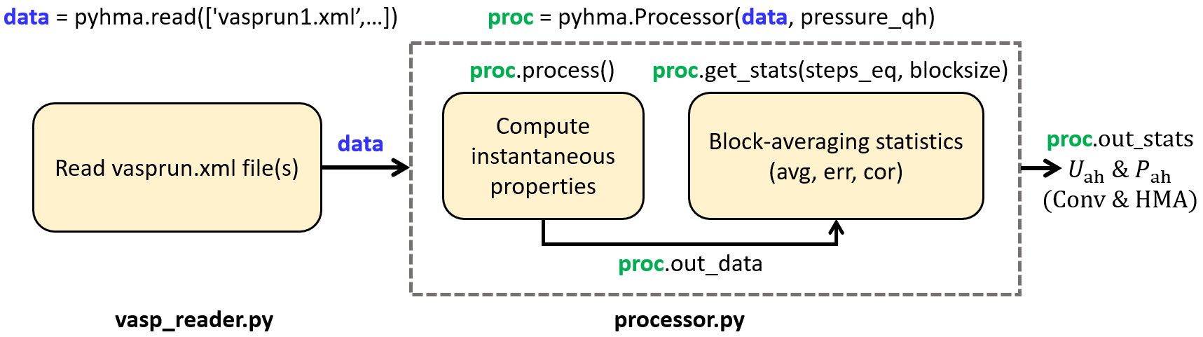
Fig. 2 Overall structure of pyHMA package.

As shown in the diagram, pyHMA post-processes VASP AIMD data in two stages: first, reading vasprun.xml output file(s) (pyhma.vasp_reader module), and then process the data to compute anharmonic properties, using conventional (Conv) and harmonically-mapped averaging (HMA) approaches (pyhma.processor module). Below is a detailed description of each stage along with an example of fcc aluminum at high pressure (\(P_{\rm lat}=114.4\) GPa; corresponds to \(V=10 A^3\)/atom) and temperature (\(1000\) K).

Attention

It is worth emphasizing here that \(U_{\rm lat}\) , \(P_{\rm lat}\) , and \(P_{\rm qh}\) inputs needed for the anharmonic calculations (see Table 1) must be obtained using the same setting with with AIMD (e.g., system size, DFT parameters, etc.) in order to ensure having the same potential-energy surface.
However, lattice and quasiharmonic contributions needed for computing the full property (lat+qh+ah) should be obtained from separate calculations as those components can converge at a different rates from the anharmonic one. The full property \(X\) can be then decomposed to \(X = X^{*}_{\rm lat} + X^{*}_{\rm qh} + X_{\rm ah}\), where the asterisk refers to using different DFT setting.
To summarize points 1 and 2 above: \(X_{\rm lat}\) and \(X_{\rm qh}\) used as inputs to pyHMA should not be used as the lat and qh contributions of the full property. On the other hand, \(X^{*}_{\rm lat}\) and \(X^{*}_{\rm qh}\) used for computing the full property should not be used as the lat and qh input parameters for pyHMA. Mixing between these two uses will result in inconsistent and inaccurate results.

1. Interactive usage¶

Reading

In this stage, pyhma.vasp_reader.read() function parses vasprun.xml AIMD simulation file and returns a data dictionary with simulation information to be processed in the second stage. In the below example, the AIMD simulation consists of two consecutive runs of the same simulation, where the initial configuration of the first run is the fcc lattice positions.

>>> import pyhma
>>> data = pyhma.read(['vasprun-1.xml', 'vasprun-2.xml'])

The data dictionary contains the following keys:

box_row_vecs (Å): box edge row vectors

num_atoms: total number of atoms

volume_atom (Å^3/atom): average volume per atom

basis: list of atomic fractional positions of first configuration

position: instantaneous atomic fractional positions

force (eV/Å): instantaneous atomic forces

energy (eV/atom): instantaneous potential energy (E0)

pressure (GPa): instantaneous pressure

pressure_ig (GPa): ideal gas pressure

timestep (fs): MD timestep

temperature (K): NVT set temperature

This function also takes optional arguments: raw_files, force_tol, and verbose. By setting raw_files=True (default is False), the following .dat files will be generated, which contain raw data from vasprun.xml file(s). These files are only for diagnostics purposes, and not used in the process stage.

poscar_eq.dat: initial (must be the equilibrium) POSCAR file (in fractional coordinates)

energy.dat: instantaneous potential energy, E0 (in eV/atom)

pressure.dat: instantaneous pressure (in GPa)

posfor.dat: instantaneous atomic positions and forces (in Å and eV/Å)

The second argument (force_tol) is the maximum force allowed on any atom in the initial configuration (default is 0.001 eV/Å). This is used to make sure the initial configuration is the minimized (or, equilibrium). If this condition is not matched, the function will be interrupted and prints a warning with a list of atoms having large initial forces.

To print the lattice vectors, and the initial atomic positions and forces, you can add verbose=True (default is False) to the arguments.

Below is the output resulted from using all optional arguments:

>>> data = pyhma.read(['vasprun-1.xml', 'vasprun-2.xml'], raw_files=True, force_tol=0.002, verbose=True)

Reading vasprun-1.xml vasprun-2.xml
==============================================
 first configuration data from vasprun-1.xml
 ----------------------------------------------
atoms (total)
 Box edge (row) vectors
83990379   0.00000000   0.00000000
00000000   6.83990379   0.00000000
00000000   0.00000000   6.83990379

 atom       xyz (direct) coordinates (A)                   xyz forces (eV/A)
  0.00000000   0.00000000   0.00000000      0.00000098   0.00000047  -0.00000207
  0.50000000   0.00000000   0.00000000     -0.00000114  -0.00000068  -0.00000010
  0.00000000   0.50000000   0.00000000      0.00000092  -0.00000001   0.00000009
  0.50000000   0.50000000   0.00000000     -0.00000075   0.00000133   0.00000002
  0.00000000   0.00000000   0.50000000      0.00000156  -0.00000124   0.00000148
  0.50000000   0.00000000   0.50000000     -0.00000228  -0.00000113   0.00000060
  0.00000000   0.50000000   0.50000000      0.00000058   0.00000088  -0.00000025
  0.50000000   0.50000000   0.50000000     -0.00000022   0.00000147   0.00000020
  0.25000000   0.25000000   0.00000000      0.00000626   0.00000445   0.00000093
  0.75000000   0.25000000   0.00000000     -0.00000698   0.00000368  -0.00000093
  0.25000000   0.75000000   0.00000000      0.00000876  -0.00000401  -0.00000012
  0.75000000   0.75000000   0.00000000     -0.00000828  -0.00000414  -0.00000230
  0.25000000   0.25000000   0.50000000      0.00000749   0.00000298  -0.00000160
  0.75000000   0.25000000   0.50000000     -0.00000890   0.00000465   0.00000053
  0.25000000   0.75000000   0.50000000      0.00000879  -0.00000420   0.00000048
  0.75000000   0.75000000   0.50000000     -0.00000810  -0.00000479   0.00000260
  0.00000000   0.25000000   0.25000000      0.00000300   0.00000494   0.00000561
  0.50000000   0.25000000   0.25000000     -0.00000351   0.00000432   0.00000600
  0.00000000   0.75000000   0.25000000      0.00000149  -0.00000550   0.00000703
  0.50000000   0.75000000   0.25000000     -0.00000171  -0.00000398   0.00000669
  0.00000000   0.25000000   0.75000000      0.00000072   0.00000397  -0.00000567
  0.50000000   0.25000000   0.75000000     -0.00000041   0.00000300  -0.00000674
  0.00000000   0.75000000   0.75000000     -0.00000135  -0.00000323  -0.00000732
  0.50000000   0.75000000   0.75000000      0.00000067  -0.00000412  -0.00000650
  0.25000000   0.00000000   0.25000000      0.00000892   0.00000095   0.00000758
  0.75000000   0.00000000   0.25000000     -0.00000866  -0.00000109   0.00000571
  0.25000000   0.50000000   0.25000000      0.00000780  -0.00000037   0.00000582
  0.75000000   0.50000000   0.25000000     -0.00000778   0.00000087   0.00000677
  0.25000000   0.00000000   0.75000000      0.00000777  -0.00000093  -0.00000665
  0.75000000   0.00000000   0.75000000     -0.00000764  -0.00000253  -0.00000547
  0.25000000   0.50000000   0.75000000      0.00000795   0.00000070  -0.00000629
  0.75000000   0.50000000   0.75000000     -0.00000705   0.00000248  -0.00000653

  Reading vasprun-1.xml  ( 1 out of 2 )
  Reading vasprun-2.xml  ( 2 out of 2 )
>>>

Note

The read() function can handle incomplete vasprun.xml file(s) generated from interrupted AIMD runs (by the user, or due to some time constraint). The was possible with using the recovery option of LXML parser.
If your MD simulation starts from a thermalized/equilibrated (not lattice) configuration, you can just run a single-point energy calculation on the lattice configuration (using the same DFT parameters used with AIMD) and use the output as your vasprun-1.xml input to pyHMA, followed by your thermalized vasprun.xml files.

Processing

In this stage, the data from previous step are processed to compute anharmonic properties. This is done, first, by creating a processor instance (proc) of the pyhma.processor.Processor() class, using the data dictionary and the quasiharmonic pressure (GPa) at the given \(V\) and \(T\). The class takes one optional argument, meV, to specify whether to report the energy results in meV (meV=True) or eV (meV=False, default). At this point, the proc object carries the same information exist in the data dictionary.

>>> proc = pyhma.Processor(data, pressure_qh=4.94154, meV=True)

Then, the instantaneous properties are obtained by calling the pyhma.processor.Processor.process() method, which takes two optional arguments: steps_tot and verbose. The steps_tot is the total number of MD steps to be used for ensemble averages (default is all steps found in vasprun.xml) and the verbose (default is False) directs pyHMA to print information while running. The output is saved to a 2D array (proc.out_data attribute) of length equal to all MD steps (or, steps_tot if set) and contains four columns: Conv and HMA anharmonic energies and pressures.

>>> proc.process(steps_tot=10000, verbose=True)

   Simulation data
   ===============
    Set temperature       (K): 1000.00000
    Volume         (A^3/atom):   10.00000
    MD timestep          (fs):    2.00000
    Lattice energy  (eV/atom):   -2.21324
    Harmonic energy (eV/atom):    0.12522
    Lattice pressure    (GPa):  114.44281
    Harmonic pressure   (GPa):    4.94525

    Found 11036  total MD steps
    Using 10000  user-set MD steps

    Computing instantaneous properties ...

The method also generates energy_ah.out and pressure_ah.out output files for the instantaneous anharmonic energy (eV/atom; or meV/atom if meV=True) and pressure (GPa), respectively. Each file contains three columns; time (in fs), Conv, and HMA estimates of the property. This data is plotted below.

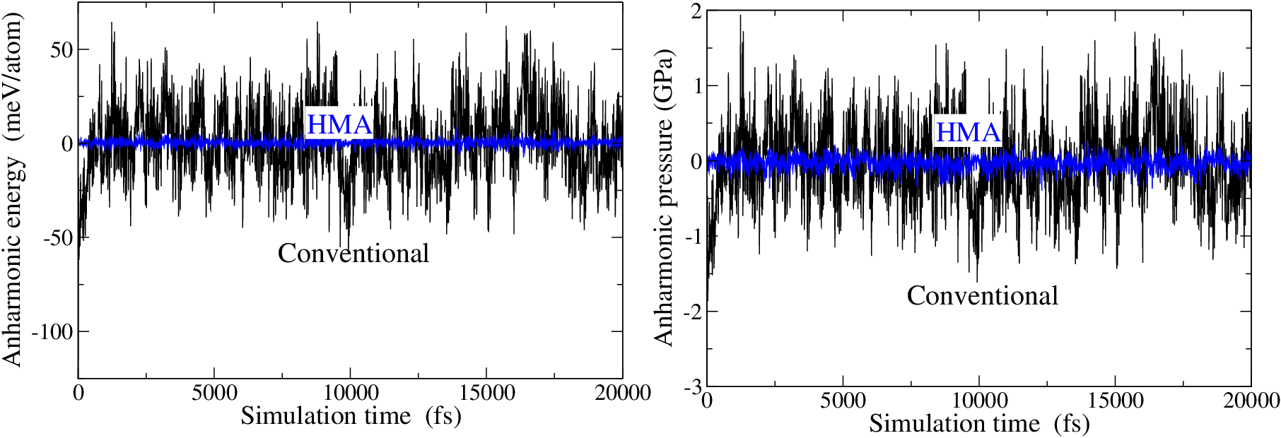
Fig. 3 Time vartaion of the anharmonic energy (energy_ah.out) and pressure (pressure_ah.out).

Lastly, ensemble statistics (average, uncertainty, and block correlation) are obtained using block averaging technique. This is done by invoking the pyhma.processor.Processor.get_stats() method, which takes two required arguments (steps_eq and blocksize) and one optional argument (verbose). The steps_eq is the number of MD steps used for equilibaration and blocksize is the number of MD steps in each block used for block averaging; so, steps_tot/blocksize is the number of blocks to be used. If True, the verbose flag will direct pyHMA to print samples information.

The method returns the statistics output in a form of a dictionary (stats) of four entries: Conv and HMA anharmonic energies (e_ah_conv and e_ah_hma) and pressures (p_ah_conv and p_ah_hma), each with three elements of average (avg), uncertainty (err), and adjacent blocks correlation (cor). The output can be presented in a more user-friendly format by using pyhma.processor.Processor.print_stats() method, which yields the output shown below.

>>> stats = proc.get_stats(steps_eq=1000, blocksize=90, verbose=True)

Block averaging statistics
==========================
 9000 production steps (after 1000 equilibration steps)
 100 blocks (blocksize = 90  steps)

 Computing statistics ...

>>> proc.print_stats(stats)

 e_ah_conv (meV/atom):    2.10911 +/- 1.1e+00    cor: 0.35
 e_ah_hma  (meV/atom):    0.42650 +/- 4.3e-02    cor: 0.11
 p_ah_conv      (GPa):    0.01371 +/- 3.1e-02    cor: 0.36
 p_ah_hma       (GPa):   -0.03419 +/- 4.1e-03    cor: 0.26

Note

The correlation should be as small as possible (less than \(\lessapprox 0.2\)) to ensure accurate estimate of uncertainty. Although increasing the blocksize reduces the correlations, the number of blocks should be large enough (\(\gtrapprox 50\)) to yield meaningful statistics.
The Conv and HMA should be statistically consistent, as long as the results are converged with respect to timestep. However, the above example has inconsistent results due to using relatively large timestep (\(\Delta t=2\) fs), though the HMA estimate is still accurate as it converges faster than Conv (see our JCP2018 work for details).

2. pyhma script¶

Anharmonic properties can be computed in one step from the command-line using pyhma script, which uses the same arguments as those used above, except for the use of r and v short forms of raw_files and verbose options, respectively. The usage of pyhma is given here, where the square brackets represent optional keys:

$ # Usage:
$ # pyhma --pressure_qh=qh pressure (GPa) --steps_eq=equilib. steps --blocksize=block size
$ #      [--steps_tot=used steps] [--force_tol=force tolerance] [--raw_files|-r] [--meV]
$ #      [--verbose|-v] vasprun-1.xml vasprun-2.xml ...

Using the pyhma script (with default option) to compute anharmonic energy and pressure of the above fcc aluminum example yields:

$ pyhma --pressure_qh=4.94525 --steps_eq=1000 --steps_tot=10000 --blocksize=90  -r --meV
        vasprun-1.xml  vasprun-2.xml

  e_ah_conv (meV/atom):    2.10911 +/- 1.1e+00    cor: 0.35
  e_ah_hma  (meV/atom):    0.42650 +/- 4.3e-02    cor: 0.11
  p_ah_conv      (GPa):    0.01371 +/- 3.1e-02    cor: 0.36
  p_ah_hma       (GPa):   -0.03419 +/- 4.1e-03    cor: 0.26

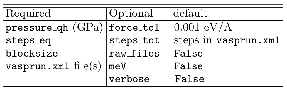
3. Parameters table¶

The Table below gives a summary of both required and optional arguments used by pyHMA.