Application to Crystals

For crystalline systems, a reference for mapping can be chosen to be non-interacting harmonic system, or Einstein crystal (EC). Using the offset from the lattice sites (i.e., \(r-r_{\rm lattice}\)) to represent our coordinate \(x\), the potential energy for each dof is then given by

\[u^{\rm ref} = \alpha(\lambda) x^2\]

hence, the free energy is given by

\[a^{\rm ref} = \frac{1}{2} \ln \left(\alpha(\lambda)/\pi\right)\]

Accordingly, \(f^{\rm ref} = -2 \alpha(\lambda) x\;\) , \(\; I=- \alpha(\lambda) x^2\), and \(g=(\partial_{\nu}\alpha)\left[ x^2 - 1/2\alpha\right]\). Requiring the mapping velocity to vanish when atoms are at their lattice sites; i.e., \({\dot x}^{\nu} =0\) at \(x = 0\), the solution of the velocity mapping equation is reduced to

\[\begin{split}{\dot x}^{\nu} &=& \; e^{-I(x)} \int_{0}^{x} g \; e^{I(x)}{\rm d}x \\ &=& \; e^{\alpha(\lambda) x^2} \int_{0}^{x} g \; e^{-\alpha(\lambda) x^2}{\rm d}x \\ &=& \; - \frac{\partial_{\nu} \alpha}{2 \alpha} \; x\end{split}\]

We will now consider two cases: temperature and volume free energy derivative; or energy and pressure, consequently. Note that all energy quantities (and its derivatives, like forces) are multiplied by \(\beta\); hence, the force constant \(\alpha \rightarrow \beta\alpha\), where \(\alpha\) is now temperature independent.

• case 1: \(\nu = \beta\)

\[\partial_{\beta} (\beta\alpha) = \alpha\]

hence,

\[{\dot x}^{\beta} = -\frac{1}{2\beta} \; x\]

• case 2: \(\nu = V\)

Here, we need to use the \(L\)-scaled coordinates (i.e., \(x\rightarrow x/L\)); hence \(\alpha \rightarrow L^2 \beta\alpha = V^{2/3}\beta\alpha(V)\)

\[\begin{split}{\dot x}^{V} &=& - \frac{1}{2} \frac{\partial_{\nu} (V^{2/3}\alpha(V))}{V^{2/3}\alpha(V)} \; x \\ &=& \left(-\frac{1}{2} \frac{\partial_{V}\alpha(V)}{\alpha(V)} - \frac{1}{3V}\right) \; x \\ &=& \left(\beta\, p^{\rm harm}- \frac{1}{3V}\right) \; x\end{split}\]

Where \(p^{\rm harm}\) is the harmonic pressure per each dof. For more details you can refer to our PRE and JCTC work.

Anharmonic energy

Conventional (no mapping):

\[U^{\rm ah} = \left< U \right> - \frac{d(N-1)}{2} k_{\rm B} T - U^{\rm lat}\]

Mapped averaging (Einstein crystal reference):

\[U^{\rm ah} = \left< U + \frac{1}{2} {\bf F}\cdot\Delta{\bf r}\right> - U^{\rm lat}\]

Anharmonic pressure

Conventional (uniform scaling):

\[P^{\rm ah} = \left< P^{\rm vir} \right> + \rho k_{\rm B}T - P^{\rm qh} - P^{\rm lat}\]

Mapped averaging (Einstein crystal reference):

\[P^{\rm ah} = \left< P^{\rm vir} + c \; {\bf F}\cdot\Delta{\bf r} \right> - P^{\rm lat}\]

where \(c\) is a constant and given by, \(c = \frac{\beta P^{\rm qh} - \rho}{d\left(N-1\right)}\)

The formulas for both anharmonic energy and pressure are summarized in Figure 1.

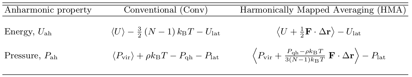
Fig. 1 Conventional and HMA formulas for anharmonic energy and pressure.

Equivalence of Conv and HMA

The equivalence between both conventional and mapped-averaging expressions can be easily seen by recognizing this equality for crystalline systems:

\[\left<{\bf F}\cdot\Delta{\bf r} \right> = - d\left(N-1\right) k_{\rm B} T\]

Plugging this expression into the HMA expressions yields the conventional average expression.

Proof:

The general expression for the configurational partition function is given by:

\[Q = \int e^{-\beta U} {\rm d} {\bf x}\]

For crystalline systems, we use \(\Delta {\bf x} \equiv {\bf x} - {\bf x}^{\rm lat}\)

\[Q = \int_{\rm WS} e^{-\beta U} \, {\rm d}^{dN}\Delta x\]

Where the integration is carried out withing the Wigner-Seitz (WS) volume of each atom. This can be written as

\[Q = \int_{\rm WS} {\rm d}^{dN-1}\Delta x \; \int_{\rm WS} e^{-\beta U} \, {\rm d} \Delta x_1\]

Using integration by parts:

\[Q = \int_{\rm WS} \; \left[\Delta x_1 e^{-\beta U}\right]_{\Delta x_1^{\rm min}}^{\Delta x_1^{\rm max}} {\rm d}^{dN-1}\Delta x \;\; -\beta \int_{\rm WS} F_1 \Delta x_1 \; e^{-\beta U} {\rm d}^{dN}\Delta x\]

The surface (first) term on the right-hand side vanishes due to large values of \(U\) at the surface of the WS volume. Dividing by Q, we finally get:

\[\left<F_1 \Delta x_1 \right> = - k_{\rm B} T\]

For \(d(N-1)\) degrees-of-freedom, we get: \(\left<{\bf F}\cdot\Delta{\bf r} \right> = - d\left(N-1\right) k_{\rm B} T\)